Back Testing - roboquant

If you have a Google account, you can run this Jupyter Notebook on Google Colab:

In this tutorial, we will walk through the core components of a backtest:

Environment Setup: Installing and configuring the library.
Feed: Getting historical market data.
Strategy: Defining the logic for buying and selling.
Run: Executing the backtest and viewing results.
Visualization: Analyzing the performance.

1. Setup and Imports¶

First, we install the package and then import the library. Roboquant is published on PyPI like most other Python packages, so installing it is straight forward.

We also set a visual style for our charts to make them more readable.

# Install roboquant
%pip install --quiet --upgrade roboquant

Note: you may need to restart the kernel to use updated packages.

import roboquant as rq

rq.set_light_style()
# uncommon following line if you prefer dark styled charts
# rq.set_dark_style()

2. The Data Feed¶

A roboquant Feed is the data source used by a backtest. It provides historical market data, such as prices and other market metrics, for one or more assets over time.

During a backtest, the feed is processed in chronological order, and each time step is passed to the strategy so it can decide whether to generate a signal.

In this notebook, we use rq.feeds.YahooFeed.us_stocks_10(), which downloads a small basket of popular US stocks from Yahoo Finance. This makes it easy to test a strategy on real market data without preparing your own dataset manually.

feed = rq.feeds.YahooFeed.us_stocks_10()

3. Strategy and Execution¶

A strategy in roboquant is a reusable decision engine that receives market data for each time step and decides whether to generate a buy, or sell signal. Strategies can be built from simple rules, technical indicators, or custom logic, and they are typically evaluated against a feed during a backtest.

For example, EMACrossover is a built-in strategy that compares a fast and slow exponential moving average. When the fast EMA crosses above the slow EMA, it may signal a long entry; when it crosses below, it may signal an exit or short position. This makes it a classic trend-following approach and a good starting point for exploring roboquant’s strategy framework.

You can create a strategy instance and run it against the feed to evaluate performance over historical data.

strategy = rq.strategies.EMACrossover()

4. Run¶

The run function connects our feed to the strategy and simulates trading, returning an Account object that holds the results.

The backtest processes the feed chronologically, allowing the strategy to generate trading signals for each time step. The resulting Account tracks portfolio value, cash, positions, executed trades.

The returned account can be inspected directly or passed to visualization tools to analyze the strategy’s results.

account = rq.run(feed, strategy)
print(account)

buying power : 1,337,454@USD
cash         : 1,337,454@USD
equity       : 3,555,617@USD
positions    : 2445@XOM, 774@MSFT, 1571@NVDA, 1053@AAPL, 906@TSLA, 545@META
trades       : 526
mkt value    : 2,218,163@USD
orders       : none
last update  : 2026-09-30 04:00:00+00:00

5. Analyzing Performance¶

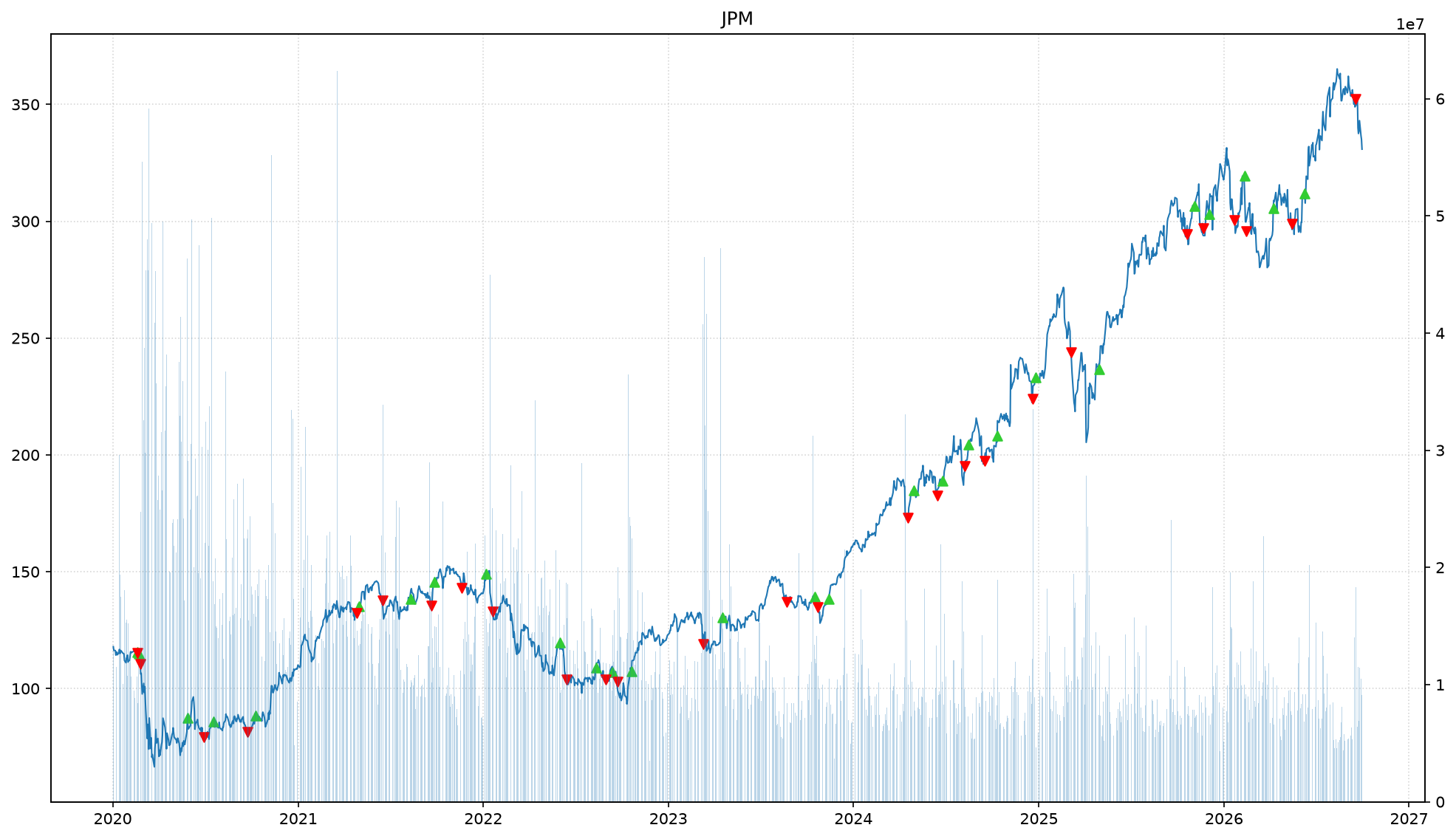
Use the feed.plot helper to inspect the price series and overlay each trade executed by the strategy for JPM. This makes it easier to visually confirm whether entries and exits align with the underlying trend and momentum.

feed.plot("JPM", trades=account.trades);